Poisson problem (MPI version)
In section Poisson problem we looked at the solution of the 3D Poisson problem (available for download at poisson3Db page) using the shared memory approach. Lets solve the same problem using the Message Passing Interface (MPI), or the distributed memory approach. We already know that using the smoothed aggregation AMG with the simple SPAI(0) smoother is working well, so we may start writing the code immediately. The following is the complete MPI-based implementation of the solver (tutorial/1.poisson3Db/poisson3Db_mpi.cpp). We discuss it in more details below.
1 2 3 4 5 6 7 8 9 10 11 12 13 14 15 16 17 18 19 20 21 22 23 24 25 26 27 28 29 30 31 32 33 34 35 36 37 38 39 40 41 42 43 44 45 46 47 48 49 50 51 52 53 54 55 56 57 58 59 60 61 62 63 64 65 66 67 68 69 70 71 72 73 74 75 76 77 78 79 80 81 82 83 84 85 86 87 88 89 90 91 92 93 94 95 96 97 98 99 100 101 102 103 104 105 106 107 108 109 110 111 112 113 114 115 116 117 118 119 120 121 122 123 124 125 126 127 128 129 130 131 132 133 134 135 136 137 | #include <vector>
#include <iostream>
#include <amgcl/backend/builtin.hpp>
#include <amgcl/adapter/crs_tuple.hpp>
#include <amgcl/mpi/distributed_matrix.hpp>
#include <amgcl/mpi/make_solver.hpp>
#include <amgcl/mpi/amg.hpp>
#include <amgcl/mpi/coarsening/smoothed_aggregation.hpp>
#include <amgcl/mpi/relaxation/spai0.hpp>
#include <amgcl/mpi/solver/bicgstab.hpp>
#include <amgcl/io/binary.hpp>
#include <amgcl/profiler.hpp>
#if defined(AMGCL_HAVE_PARMETIS)
# include <amgcl/mpi/partition/parmetis.hpp>
#elif defined(AMGCL_HAVE_SCOTCH)
# include <amgcl/mpi/partition/ptscotch.hpp>
#endif
//---------------------------------------------------------------------------
int main(int argc, char *argv[]) {
// The matrix and the RHS file names should be in the command line options:
if (argc < 3) {
std::cerr << "Usage: " << argv[0] << " <matrix.bin> <rhs.bin>" << std::endl;
return 1;
}
amgcl::mpi::init mpi(&argc, &argv);
amgcl::mpi::communicator world(MPI_COMM_WORLD);
// The profiler:
amgcl::profiler<> prof("poisson3Db MPI");
// Read the system matrix and the RHS:
prof.tic("read");
// Get the global size of the matrix:
ptrdiff_t rows = amgcl::io::crs_size<ptrdiff_t>(argv[1]);
ptrdiff_t cols;
// Split the matrix into approximately equal chunks of rows
ptrdiff_t chunk = (rows + world.size - 1) / world.size;
ptrdiff_t row_beg = std::min(rows, chunk * world.rank);
ptrdiff_t row_end = std::min(rows, row_beg + chunk);
chunk = row_end - row_beg;
// Read our part of the system matrix and the RHS.
std::vector<ptrdiff_t> ptr, col;
std::vector<double> val, rhs;
amgcl::io::read_crs(argv[1], rows, ptr, col, val, row_beg, row_end);
amgcl::io::read_dense(argv[2], rows, cols, rhs, row_beg, row_end);
prof.toc("read");
if (world.rank == 0)
std::cout
<< "World size: " << world.size << std::endl
<< "Matrix " << argv[1] << ": " << rows << "x" << rows << std::endl
<< "RHS " << argv[2] << ": " << rows << "x" << cols << std::endl;
// Compose the solver type
typedef amgcl::backend::builtin<double> DBackend;
typedef amgcl::backend::builtin<float> FBackend;
typedef amgcl::mpi::make_solver<
amgcl::mpi::amg<
FBackend,
amgcl::mpi::coarsening::smoothed_aggregation<FBackend>,
amgcl::mpi::relaxation::spai0<FBackend>
>,
amgcl::mpi::solver::bicgstab<DBackend>
> Solver;
// Create the distributed matrix from the local parts.
auto A = std::make_shared<amgcl::mpi::distributed_matrix<DBackend>>(
world, std::tie(chunk, ptr, col, val));
// Partition the matrix and the RHS vector.
// If neither ParMETIS not PT-SCOTCH are not available,
// just keep the current naive partitioning.
#if defined(AMGCL_HAVE_PARMETIS) || defined(AMGCL_HAVE_SCOTCH)
# if defined(AMGCL_HAVE_PARMETIS)
typedef amgcl::mpi::partition::parmetis<DBackend> Partition;
# elif defined(AMGCL_HAVE_SCOTCH)
typedef amgcl::mpi::partition::ptscotch<DBackend> Partition;
# endif
if (world.size > 1) {
prof.tic("partition");
Partition part;
// part(A) returns the distributed permutation matrix:
auto P = part(*A);
auto R = transpose(*P);
// Reorder the matrix:
A = product(*R, *product(*A, *P));
// and the RHS vector:
std::vector<double> new_rhs(R->loc_rows());
R->move_to_backend(typename DBackend::params());
amgcl::backend::spmv(1, *R, rhs, 0, new_rhs);
rhs.swap(new_rhs);
// Update the number of the local rows
// (it may have changed as a result of permutation):
chunk = A->loc_rows();
prof.toc("partition");
}
#endif
// Initialize the solver:
prof.tic("setup");
Solver solve(world, A);
prof.toc("setup");
// Show the mini-report on the constructed solver:
if (world.rank == 0)
std::cout << solve << std::endl;
// Solve the system with the zero initial approximation:
int iters;
double error;
std::vector<double> x(chunk, 0.0);
prof.tic("solve");
std::tie(iters, error) = solve(*A, rhs, x);
prof.toc("solve");
// Output the number of iterations, the relative error,
// and the profiling data:
if (world.rank == 0)
std::cout
<< "Iters: " << iters << std::endl
<< "Error: " << error << std::endl
<< prof << std::endl;
}
|
In lines 4–21 we include the required components. Here we are using the
builtin (OpenMP-based) backend and the CRS tuple adapter. Next we include
MPI-specific headers that provide the distributed-memory implementation of
AMGCL algorithms. This time, we are reading the system matrix and the RHS
vector in the binary format, and include <amgcl/io/binary.hpp> header
intead of the usual <amgcl/io/mm.hpp>. The binary format is not only faster
to read, but it also allows to read the matrix and the RHS vector in chunks,
which is what we need for the distributed approach.
After checking the validity of the command line parameters, we initialize the MPI context and communicator in lines 31–32:
31 32 | amgcl::mpi::init mpi(&argc, &argv);
amgcl::mpi::communicator world(MPI_COMM_WORLD);
|
The amgcl::mpi::init is a convenience RAII wrapper for
MPI_Init(). It will call MPI_Finalize() in the destructor
when its instance (mpi) goes out of scope at the end of the program. We
don’t have to use the wrapper, but it simply makes things easier.
amgcl::mpi::communicator is an equally thin wrapper for
MPI_Comm. amgcl::mpi::communicator and MPI_Comm may be
used interchangeably both with the AMGCL MPI interface and the native MPI
functions.
The system has to be divided (partitioned) between multiple MPI processes. The simplest way to do this is presented on the following figure:
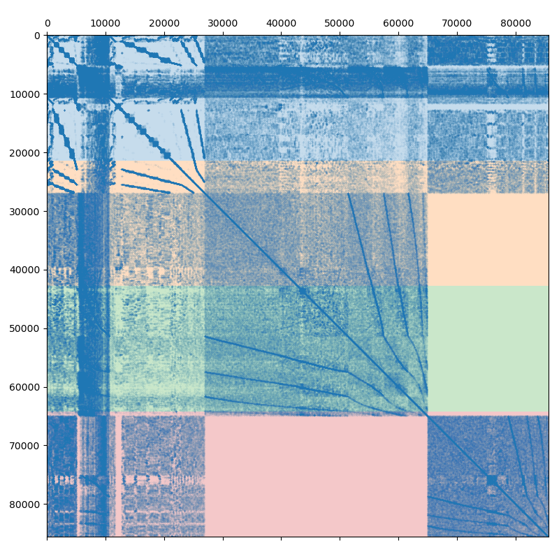
Fig. 2 Poisson3Db matrix partitioned between the 4 MPI processes
Assuming we are using 4 MPI processes, the matrix is split into 4 continuous chunks of rows, so that each MPI process owns approximately 25% of the matrix. This works well enough for a small number of processes, but as the size of the compute cluster grows, the simple partitioning becomes less and less efficient. Creating efficient partitioning is outside of AMGCL scope, but AMGCL does provide wrappers for the ParMETIS and PT-SCOTCH libraries specializing in this. The difference between the naive and the optimal partitioning is demonstrated on the next figure:
(Source code, png, hires.png, pdf)
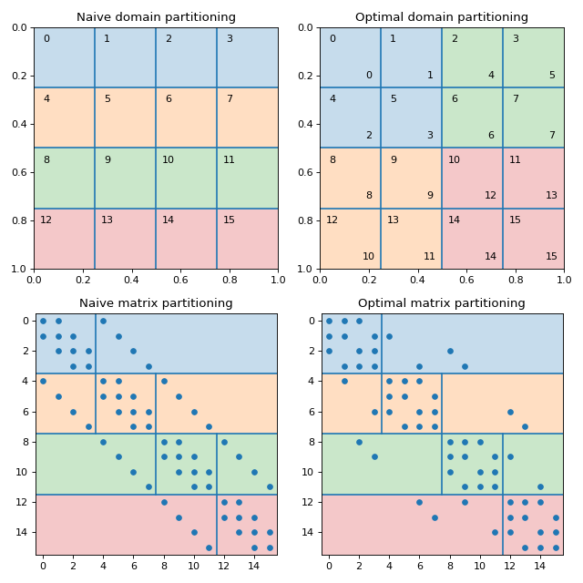
Fig. 3 Naive vs optimal partitioning of a \(4\times4\) grid between 4 MPI processes.
The figure shows the finite-diffrence discretization of a 2D Poisson problem on a \(4\times4\) grid in a unit square. The nonzero pattern of the system matrix is presented on the lower left plot. If the grid nodes are numbered row-wise, then the naive partitioning of the system matrix for the 4 MPI processes is shown on the upper left plot. The subdomains belonging to each of the MPI processes correspond to the continuous ranges of grid node indices and are elongated along the X axis. This results in high MPI communication traffic, as the number of the interface nodes is high relative to the number of interior nodes. The upper right plot shows the optimal partitioning of the domain for the 4 MPI processes. In order to keep the rows owned by a single MPI process adjacent to each other (so that each MPI process owns a continuous range of rows, as required by AMGCL), the grid nodes have to be renumbered. The labels in the top left corner of each grid node show the original numbering, and the lower-rigth labels show the new numbering. The renumbering of the matrix may be expressed as the permutation matrix \(P\), where \(P_{ij} = 1\) if the \(j\)-th unknown in the original ordering is mapped to the \(i\)-th unknown in the new ordering. The reordered system may be written as
The reordered matrix \(P^T A P\) and the corresponding partitioning are shown on the lower right plot. Note that off-diagonal blocks on each MPI process have as much as twice fewer non-zeros compared to the naive partitioning of the matrix. The solution \(x\) in the original ordering may be obtained with \(x = P y\).
In lines 37–54 we read the system matrix and the RHS vector using the naive ordering (a nicer ordering of the unknowns will be determined later):
37 38 39 40 41 42 43 44 45 46 47 48 49 50 51 52 53 54 | // Read the system matrix and the RHS:
prof.tic("read");
// Get the global size of the matrix:
ptrdiff_t rows = amgcl::io::crs_size<ptrdiff_t>(argv[1]);
ptrdiff_t cols;
// Split the matrix into approximately equal chunks of rows
ptrdiff_t chunk = (rows + world.size - 1) / world.size;
ptrdiff_t row_beg = std::min(rows, chunk * world.rank);
ptrdiff_t row_end = std::min(rows, row_beg + chunk);
chunk = row_end - row_beg;
// Read our part of the system matrix and the RHS.
std::vector<ptrdiff_t> ptr, col;
std::vector<double> val, rhs;
amgcl::io::read_crs(argv[1], rows, ptr, col, val, row_beg, row_end);
amgcl::io::read_dense(argv[2], rows, cols, rhs, row_beg, row_end);
prof.toc("read");
|
First, we read the total (global) number of rows in the matrix from the binary
file using the amgcl::io::crs_size() function. Next, we divide the
global rows between the MPI processes, and read our portions of the matrix and
the RHS using amgcl::io::read_crs() and
amgcl::io::read_dense() functions. The row_beg and row_end
parameters to the functions specify the regions (in row numbers) to read. The
column indices are kept in global numbering.
In lines 62–72 we define the backend and the solver types:
62 63 64 65 66 67 68 69 70 71 72 | // Compose the solver type
typedef amgcl::backend::builtin<double> DBackend;
typedef amgcl::backend::builtin<float> FBackend;
typedef amgcl::mpi::make_solver<
amgcl::mpi::amg<
FBackend,
amgcl::mpi::coarsening::smoothed_aggregation<FBackend>,
amgcl::mpi::relaxation::spai0<FBackend>
>,
amgcl::mpi::solver::bicgstab<DBackend>
> Solver;
|
The structure of the solver is the same as in the shared memory case in the
Poisson problem tutorial, but we are using the components from the
amgcl::mpi namespace. Again, we are using the mixed-precision approach and
the preconditioner backend is defined with a single-precision value type.
In lines 74–76 we create the distributed matrix from the local strips read by each of the MPI processes:
74 75 76 | // Create the distributed matrix from the local parts.
auto A = std::make_shared<amgcl::mpi::distributed_matrix<DBackend>>(
world, std::tie(chunk, ptr, col, val));
|
We could directly use the tuple of the CRS arrays std::tie(chunk, ptr, col,
val) to construct the solver (the distributed matrix would be created behind
the scenes for us), but here we need to explicitly create the matrix for a
couple of reasons. First, since we are using the mixed-precision approach, we
need the double-precision distributed matrix for the solution step. And second,
the matrix will be used to repartition the system using either ParMETIS or
PT-SCOTCH libraries in lines 78–110:
78 79 80 81 82 83 84 85 86 87 88 89 90 91 92 93 94 95 96 97 98 99 100 101 102 103 104 105 106 107 108 109 110 | // Partition the matrix and the RHS vector.
// If neither ParMETIS not PT-SCOTCH are not available,
// just keep the current naive partitioning.
#if defined(AMGCL_HAVE_PARMETIS) || defined(AMGCL_HAVE_SCOTCH)
# if defined(AMGCL_HAVE_PARMETIS)
typedef amgcl::mpi::partition::parmetis<DBackend> Partition;
# elif defined(AMGCL_HAVE_SCOTCH)
typedef amgcl::mpi::partition::ptscotch<DBackend> Partition;
# endif
if (world.size > 1) {
prof.tic("partition");
Partition part;
// part(A) returns the distributed permutation matrix:
auto P = part(*A);
auto R = transpose(*P);
// Reorder the matrix:
A = product(*R, *product(*A, *P));
// and the RHS vector:
std::vector<double> new_rhs(R->loc_rows());
R->move_to_backend(typename DBackend::params());
amgcl::backend::spmv(1, *R, rhs, 0, new_rhs);
rhs.swap(new_rhs);
// Update the number of the local rows
// (it may have changed as a result of permutation):
chunk = A->loc_rows();
prof.toc("partition");
}
#endif
|
We determine if either ParMETIS or PT-SCOTCH is available in lines 81–86,
and use the corresponding wrapper provided by the AMGCL. The wrapper computes
the permutation matrix \(P\), which is used to reorder both the system
matrix and the RHS vector. Since the reordering may change the number of rows
owned by each MPI process, we update the number of local rows stored in the
chunk variable.
112 113 114 115 116 117 118 119 120 121 122 123 124 125 126 127 128 | // Initialize the solver:
prof.tic("setup");
Solver solve(world, A);
prof.toc("setup");
// Show the mini-report on the constructed solver:
if (world.rank == 0)
std::cout << solve << std::endl;
// Solve the system with the zero initial approximation:
int iters;
double error;
std::vector<double> x(chunk, 0.0);
prof.tic("solve");
std::tie(iters, error) = solve(*A, rhs, x);
prof.toc("solve");
|
At this point we are ready to initialize the solver (line 115), and solve the
system (line 128). Here is the output of the compiled program. Note that the
environment variable OMP_NUM_THREADS is set to 1 in order to not
oversubscribe the available CPU cores:
$ export OMP_NUM_THREADS=1
$ mpirun -np 4 ./poisson3Db_mpi poisson3Db.bin poisson3Db_b.bin
World size: 4
Matrix poisson3Db.bin: 85623x85623
RHS poisson3Db_b.bin: 85623x1
Partitioning[ParMETIS] 4 -> 4
Type: BiCGStab
Unknowns: 21671
Memory footprint: 1.16 M
Number of levels: 3
Operator complexity: 1.20
Grid complexity: 1.08
level unknowns nonzeros
---------------------------------
0 85623 2374949 (83.06%) [4]
1 6377 450473 (15.75%) [4]
2 401 34039 ( 1.19%) [4]
Iters: 24
Error: 6.09835e-09
[poisson3Db MPI: 1.273 s] (100.00%)
[ self: 0.044 s] ( 3.49%)
[ partition: 0.626 s] ( 49.14%)
[ read: 0.012 s] ( 0.93%)
[ setup: 0.152 s] ( 11.92%)
[ solve: 0.439 s] ( 34.52%)
Similarly to how it was done in the Poisson problem section, we can use the GPU backend in order to speed up the solution step. Since the CUDA backend does not support the mixed-precision approach, we will use the VexCL backend, which allows to employ CUDA, OpenCL, or OpenMP compute devices. The source code (tutorial/1.poisson3Db/poisson3Db_mpi_vexcl.cpp) is very similar to the version using the builtin backend and is shown below with the differences highlighted.
1 2 3 4 5 6 7 8 9 10 11 12 13 14 15 16 17 18 19 20 21 22 23 24 25 26 27 28 29 30 31 32 33 34 35 36 37 38 39 40 41 42 43 44 45 46 47 48 49 50 51 52 53 54 55 56 57 58 59 60 61 62 63 64 65 66 67 68 69 70 71 72 73 74 75 76 77 78 79 80 81 82 83 84 85 86 87 88 89 90 91 92 93 94 95 96 97 98 99 100 101 102 103 104 105 106 107 108 109 110 111 112 113 114 115 116 117 118 119 120 121 122 123 124 125 126 127 128 129 130 131 132 133 134 135 136 137 138 139 140 141 142 143 144 145 146 147 148 149 150 151 152 153 154 155 | #include <vector>
#include <iostream>
#include <amgcl/backend/vexcl.hpp>
#include <amgcl/adapter/crs_tuple.hpp>
#include <amgcl/mpi/distributed_matrix.hpp>
#include <amgcl/mpi/make_solver.hpp>
#include <amgcl/mpi/amg.hpp>
#include <amgcl/mpi/coarsening/smoothed_aggregation.hpp>
#include <amgcl/mpi/relaxation/spai0.hpp>
#include <amgcl/mpi/solver/bicgstab.hpp>
#include <amgcl/io/binary.hpp>
#include <amgcl/profiler.hpp>
#if defined(AMGCL_HAVE_PARMETIS)
# include <amgcl/mpi/partition/parmetis.hpp>
#elif defined(AMGCL_HAVE_SCOTCH)
# include <amgcl/mpi/partition/ptscotch.hpp>
#endif
//---------------------------------------------------------------------------
int main(int argc, char *argv[]) {
// The matrix and the RHS file names should be in the command line options:
if (argc < 3) {
std::cerr << "Usage: " << argv[0] << " <matrix.bin> <rhs.bin>" << std::endl;
return 1;
}
    amgcl::mpi::init mpi(&argc, &argv);
    amgcl::mpi::communicator world(MPI_COMM_WORLD);
// Create VexCL context. Use vex::Filter::Exclusive so that different MPI
// processes get different GPUs. Each process gets a single GPU:
vex::Context ctx(vex::Filter::Exclusive(vex::Filter::Count(1)));
for(int i = 0; i < world.size; ++i) {
// unclutter the output:
if (i == world.rank)
std::cout << world.rank << ": " << ctx.queue(0) << std::endl;
MPI_Barrier(world);
}
// The profiler:
amgcl::profiler<> prof("poisson3Db MPI(VexCL)");
    // Read the system matrix and the RHS:
    prof.tic("read");
    // Get the global size of the matrix:
    ptrdiff_t rows = amgcl::io::crs_size<ptrdiff_t>(argv[1]);
    ptrdiff_t cols;

    // Split the matrix into approximately equal chunks of rows
    ptrdiff_t chunk = (rows + world.size - 1) / world.size;
    ptrdiff_t row_beg = std::min(rows, chunk * world.rank);
    ptrdiff_t row_end = std::min(rows, row_beg + chunk);
    chunk = row_end - row_beg;

    // Read our part of the system matrix and the RHS.
    std::vector<ptrdiff_t> ptr, col;
    std::vector<double> val, rhs;
    amgcl::io::read_crs(argv[1], rows, ptr, col, val, row_beg, row_end);
    amgcl::io::read_dense(argv[2], rows, cols, rhs, row_beg, row_end);
    prof.toc("read");
// Copy the RHS vector to the backend:
vex::vector<double> f(ctx, rhs);
if (world.rank == 0)
std::cout
<< "World size: " << world.size << std::endl
<< "Matrix " << argv[1] << ": " << rows << "x" << rows << std::endl
<< "RHS " << argv[2] << ": " << rows << "x" << cols << std::endl;
// Compose the solver type
typedef amgcl::backend::vexcl<double> DBackend;
typedef amgcl::backend::vexcl<float> FBackend;
typedef amgcl::mpi::make_solver<
amgcl::mpi::amg<
FBackend,
amgcl::mpi::coarsening::smoothed_aggregation<FBackend>,
amgcl::mpi::relaxation::spai0<FBackend>
>,
amgcl::mpi::solver::bicgstab<DBackend>
> Solver;
    // Create the distributed matrix from the local parts.
    auto A = std::make_shared<amgcl::mpi::distributed_matrix<DBackend>>(
            world, std::tie(chunk, ptr, col, val));
// Partition the matrix and the RHS vector.
// If neither ParMETIS not PT-SCOTCH are not available,
// just keep the current naive partitioning.
#if defined(AMGCL_HAVE_PARMETIS) || defined(AMGCL_HAVE_SCOTCH)
# if defined(AMGCL_HAVE_PARMETIS)
typedef amgcl::mpi::partition::parmetis<DBackend> Partition;
# elif defined(AMGCL_HAVE_SCOTCH)
typedef amgcl::mpi::partition::ptscotch<DBackend> Partition;
# endif
if (world.size > 1) {
prof.tic("partition");
Partition part;
// part(A) returns the distributed permutation matrix:
auto P = part(*A);
auto R = transpose(*P);
// Reorder the matrix:
A = product(*R, *product(*A, *P));
// and the RHS vector:
vex::vector<double> new_rhs(ctx, R->loc_rows());
R->move_to_backend(typename DBackend::params());
amgcl::backend::spmv(1, *R, f, 0, new_rhs);
f.swap(new_rhs);
// Update the number of the local rows
// (it may have changed as a result of permutation):
chunk = A->loc_rows();
prof.toc("partition");
}
#endif
// Initialize the solver:
Solver::params prm;
DBackend::params bprm;
bprm.q = ctx;
prof.tic("setup");
Solver solve(world, A, prm, bprm);
prof.toc("setup");
// Show the mini-report on the constructed solver:
if (world.rank == 0)
std::cout << solve << std::endl;
// Solve the system with the zero initial approximation:
int iters;
double error;
vex::vector<double> x(ctx, chunk);
x = 0.0;
prof.tic("solve");
std::tie(iters, error) = solve(*A, f, x);
prof.toc("solve");
// Output the number of iterations, the relative error,
// and the profiling data:
if (world.rank == 0)
std::cout
<< "Iters: " << iters << std::endl
<< "Error: " << error << std::endl
<< prof << std::endl;
}
|
Basically, we replace the builtin backend with the vexcl one,
initialize the VexCL context and reference the context in the backend
parameters. The RHS and the solution vectors are need to be
transfered/allocated on the GPUs.
Below is the output of the VexCL version using the OpenCL technology. Note that
the system the tests were performed on has only two GPUs, so the test used just
two MPI processes. The environment variable OMP_NUM_THREADS was set to 2 in
order to fully utilize all available CPU cores:
$ export OMP_NUM_THREADS=2
$ mpirun -np 2 ./poisson3Db_mpi_vexcl_cl poisson3Db.bin poisson3Db_b.bin
0: GeForce GTX 960 (NVIDIA CUDA)
1: GeForce GTX 1050 Ti (NVIDIA CUDA)
World size: 2
Matrix poisson3Db.bin: 85623x85623
RHS poisson3Db_b.bin: 85623x1
Partitioning[ParMETIS] 2 -> 2
Type:             BiCGStab
Unknowns:         43255
Memory footprint: 2.31 M

Number of levels:    3
Operator complexity: 1.20
Grid complexity:     1.08

level     unknowns       nonzeros
---------------------------------
    0        85623        2374949 (83.03%) [2]
    1         6381         451279 (15.78%) [2]
    2          396          34054 ( 1.19%) [2]

Iters: 24
Error: 9.14603e-09

[poisson3Db MPI(VexCL):     1.132 s] (100.00%)
[ self:                     0.040 s] (  3.56%)
[  partition:               0.607 s] ( 53.58%)
[  read:                    0.015 s] (  1.31%)
[  setup:                   0.287 s] ( 25.31%)
[  solve:                   0.184 s] ( 16.24%)