Poisson problem
This system may be downloaded from the poisson3Db page (use the Matrix Market download option). The system matrix has 85,623 rows and 2,374,949 nonzeros (which is on average is about 27 non-zero elements per row). The matrix has an interesting structure, presented on the figure below:
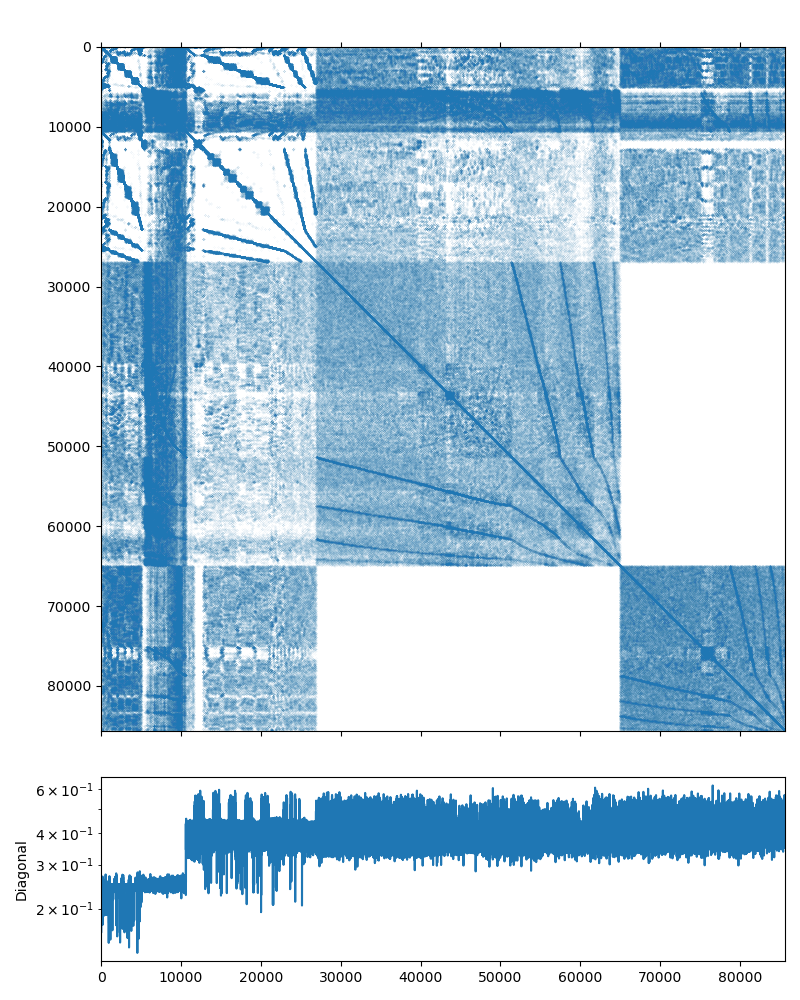
Fig. 1 Poisson3Db matrix portrait
A Poisson problem should be an ideal candidate for a solution with an AMG preconditioner, but before we start writing any code, let us check this with the examples/solver utility provided by AMGCL. It can take the input matrix and the RHS in the Matrix Market format, and allows to play with various solver and preconditioner options.
Note
The examples/solver is convenient not only for testing the systems
obtained elsewhere. You can also save your own matrix and the RHS vector
into the Matrix Market format with amgcl::io::mm_write()
function. This way you can find the AMGCL options that work for your
problem without the need to rewrite the code and recompile the program.
The default options of BiCGStab iterative solver preconditioned with a smoothed aggregation AMG (a simple diagonal SPAI(0) relaxation is used on each level of the AMG hierarchy) should work very well for a Poisson problem:
$ solver -A poisson3Db.mtx -f poisson3Db_b.mtx
Solver
======
Type:             BiCGStab
Unknowns:         85623
Memory footprint: 4.57 M

Preconditioner
==============
Number of levels:    3
Operator complexity: 1.20
Grid complexity:     1.08
Memory footprint:    58.93 M

level     unknowns       nonzeros      memory
---------------------------------------------
    0        85623        2374949     50.07 M (83.20%)
    1         6361         446833      7.78 M (15.65%)
    2          384          32566      1.08 M ( 1.14%)

Iterations: 24
Error:      8.33789e-09

[Profile:       2.351 s] (100.00%)
[  reading:     1.623 s] ( 69.01%)
[  setup:       0.136 s] (  5.78%)
[  solve:       0.592 s] ( 25.17%)
As we can see from the output, the solution converged in 24 iterations to the default relative error of 1e-8. The solver setup took 0.136 seconds and the solution time is 0.592 seconds. The iterative solver used 4.57M of memory, and the preconditioner required 58.93M. This looks like a well-performing solver already, but we can try a couple of things just in case. We can not use the simpler CG solver, because the matrix is reported as a non-symmetric on the poisson3Db page. Using the GMRES solver seems to work equally well (the solution time is just slightly lower, but the solver requires more memory to store the orthogonal vectors). The number of iterations seems to have grown, but keep in mind that each iteration of BiCGStab requires two matrix-vector products and two preconditioner applications, while GMRES only makes one of each:
$ solver -A poisson3Db.mtx -f poisson3Db_b.mtx solver.type=gmres
Solver
======
Type:             GMRES(30)
Unknowns:         85623
Memory footprint: 20.91 M

Preconditioner
==============
Number of levels:    3
Operator complexity: 1.20
Grid complexity:     1.08
Memory footprint:    58.93 M

level     unknowns       nonzeros      memory
---------------------------------------------
    0        85623        2374949     50.07 M (83.20%)
    1         6361         446833      7.78 M (15.65%)
    2          384          32566      1.08 M ( 1.14%)

Iterations: 39
Error:      9.50121e-09

[Profile:       2.282 s] (100.00%)
[  reading:     1.612 s] ( 70.66%)
[  setup:       0.135 s] (  5.93%)
[  solve:       0.533 s] ( 23.38%)
We can also try differrent relaxation options for the AMG preconditioner. But as we can see below, the simplest SPAI(0) works well enough for a Poisson problem. The incomplete LU decomposition with zero fill-in makes less iterations, but is more expensive to setup:
$ solver -A poisson3Db.mtx -f poisson3Db_b.mtx precond.relax.type=ilu0
Solver
======
Type:             BiCGStab
Unknowns:         85623
Memory footprint: 4.57 M

Preconditioner
==============
Number of levels:    3
Operator complexity: 1.20
Grid complexity:     1.08
Memory footprint:    103.44 M

level     unknowns       nonzeros      memory
---------------------------------------------
    0        85623        2374949     87.63 M (83.20%)
    1         6361         446833     14.73 M (15.65%)
    2          384          32566      1.08 M ( 1.14%)

Iterations: 12
Error:      7.99207e-09

[Profile:       2.510 s] (100.00%)
[ self:         0.005 s] (  0.19%)
[  reading:     1.614 s] ( 64.30%)
[  setup:       0.464 s] ( 18.51%)
[  solve:       0.427 s] ( 17.01%)
On the other hand, the Chebyshev relaxation has cheap setup but its application is expensive as it involves multiple matrix-vector products. So, even it requires less iterations, the overall solution time does not improve that much:
$ solver -A poisson3Db.mtx -f poisson3Db_b.mtx precond.relax.type=chebyshev
Solver
======
Type:             BiCGStab
Unknowns:         85623
Memory footprint: 4.57 M

Preconditioner
==============
Number of levels:    3
Operator complexity: 1.20
Grid complexity:     1.08
Memory footprint:    59.63 M

level     unknowns       nonzeros      memory
---------------------------------------------
    0        85623        2374949     50.72 M (83.20%)
    1         6361         446833      7.83 M (15.65%)
    2          384          32566      1.08 M ( 1.14%)

Iterations: 8
Error:      5.21588e-09

[Profile:       2.316 s] (100.00%)
[  reading:     1.607 s] ( 69.39%)
[  setup:       0.134 s] (  5.78%)
[  solve:       0.574 s] ( 24.80%)
Now that we have the feel of the problem, we can actually write some code. The complete source may be found in tutorial/1.poisson3Db/poisson3Db.cpp and is presented below:
1 2 3 4 5 6 7 8 9 10 11 12 13 14 15 16 17 18 19 20 21 22 23 24 25 26 27 28 29 30 31 32 33 34 35 36 37 38 39 40 41 42 43 44 45 46 47 48 49 50 51 52 53 54 55 56 57 58 59 60 61 62 63 64 65 66 67 68 69 70 71 72 73 74 75 76 77 78 79 80 81 82 83 84 | #include <vector>
#include <iostream>
#include <amgcl/backend/builtin.hpp>
#include <amgcl/adapter/crs_tuple.hpp>
#include <amgcl/make_solver.hpp>
#include <amgcl/amg.hpp>
#include <amgcl/coarsening/smoothed_aggregation.hpp>
#include <amgcl/relaxation/spai0.hpp>
#include <amgcl/solver/bicgstab.hpp>
#include <amgcl/io/mm.hpp>
#include <amgcl/profiler.hpp>
int main(int argc, char *argv[]) {
// The matrix and the RHS file names should be in the command line options:
if (argc < 3) {
std::cerr << "Usage: " << argv[0] << " <matrix.mtx> <rhs.mtx>" << std::endl;
return 1;
}
// The profiler:
amgcl::profiler<> prof("poisson3Db");
// Read the system matrix and the RHS:
ptrdiff_t rows, cols;
std::vector<ptrdiff_t> ptr, col;
std::vector<double> val, rhs;
prof.tic("read");
std::tie(rows, cols) = amgcl::io::mm_reader(argv[1])(ptr, col, val);
std::cout << "Matrix " << argv[1] << ": " << rows << "x" << cols << std::endl;
std::tie(rows, cols) = amgcl::io::mm_reader(argv[2])(rhs);
std::cout << "RHS " << argv[2] << ": " << rows << "x" << cols << std::endl;
prof.toc("read");
// We use the tuple of CRS arrays to represent the system matrix.
// Note that std::tie creates a tuple of references, so no data is actually
// copied here:
auto A = std::tie(rows, ptr, col, val);
// Compose the solver type
// the solver backend:
typedef amgcl::backend::builtin<double> SBackend;
// the preconditioner backend:
#ifdef MIXED_PRECISION
typedef amgcl::backend::builtin<float> PBackend;
#else
typedef amgcl::backend::builtin<double> PBackend;
#endif
typedef amgcl::make_solver<
amgcl::amg<
PBackend,
amgcl::coarsening::smoothed_aggregation,
amgcl::relaxation::spai0
>,
amgcl::solver::bicgstab<SBackend>
> Solver;
// Initialize the solver with the system matrix:
prof.tic("setup");
Solver solve(A);
prof.toc("setup");
// Show the mini-report on the constructed solver:
std::cout << solve << std::endl;
// Solve the system with the zero initial approximation:
int iters;
double error;
std::vector<double> x(rows, 0.0);
prof.tic("solve");
std::tie(iters, error) = solve(A, rhs, x);
prof.toc("solve");
// Output the number of iterations, the relative error,
// and the profiling data:
std::cout << "Iters: " << iters << std::endl
<< "Error: " << error << std::endl
<< prof << std::endl;
}
|
In lines 4–10 we include the necessary AMGCL headers:
the builtin backend uses the OpenMP threading model; the crs_tuple matrix
adaper allows to use a std::tuple of CRS arrays as an input matrix; the
amgcl::make_solver class binds together a preconditioner and an iterative
solver; amgcl::amg class is the AMG preconditioner;
amgcl::coarsening::smoothed_aggregation defines the smoothed
aggreation coarsening strategy; amgcl::relaxation::spai0 is the
sparse approximate inverse relaxation used on each level of the AMG hierarchy;
and amgcl::solver::bicgstab is the BiCGStab iterative solver.
In lines 12–13 we include the Matrix Market reader and the AMGCL profiler.
After checking the validity of the command line arguments (lines 16–20), and initializing the profiler (line 23), we read the system matrix and the RHS vector from the Matrix Market files specified on the command line (lines 30–36).
Now we are ready to actually solve the system. First, we define the backends
that we use with the iterative solver and the preconditioner (lines 44–51).
The backend have to belong to the same class (in this case,
amgcl::backend::builtin), but may have different value type
precision. Here we use a double precision backend for the iterative solver, but
choose either a double or a single precision for the preconditioner backend,
depending on whether the preprocessor macro MIXED_PRECISION was defined
during compilation. Using a single precision preconditioner may be both more
memory efficient and faster, since the iterative solvers performance is usually
memory-bound.
The defined backends are used in the solver definition (lines 53–60). Here we
are using the amgcl::make_solver class to couple the AMG
preconditioner with the BiCGStab iterative solver. We istantiate the solver in
line 64.
In line 76 we solve the system for the given RHS vector, starting with a zero
initial approximation (the x vector acts as an initial approximation on
input, and contains the solution on output).
Below is the output of the program when compiled with a double precision preconditioner. The results are close to what we have seen with the examples/solver utility above, which is a good sign:
$ ./poisson3Db poisson3Db.mtx poisson3Db_b.mtx
Matrix poisson3Db.mtx: 85623x85623
RHS poisson3Db_b.mtx: 85623x1
Solver
======
Type:             BiCGStab
Unknowns:         85623
Memory footprint: 4.57 M

Preconditioner
==============
Number of levels:    3
Operator complexity: 1.20
Grid complexity:     1.08
Memory footprint:    58.93 M

level     unknowns       nonzeros      memory
---------------------------------------------
    0        85623        2374949     50.07 M (83.20%)
    1         6361         446833      7.78 M (15.65%)
    2          384          32566      1.08 M ( 1.14%)

Iters: 24
Error: 8.33789e-09

[poisson3Db:     2.412 s] (100.00%)
[  read:         1.618 s] ( 67.08%)
[  setup:        0.143 s] (  5.94%)
[  solve:        0.651 s] ( 26.98%)
Looking at the output of the mixed precision version, it is apparent that it uses less memory for the preconditioner (43.59M as opposed to 58.93M in the double-precision case), and is slightly faster during both the setup and the solution phases:
$ ./poisson3Db_mixed poisson3Db.mtx poisson3Db_b.mtx
Matrix poisson3Db.mtx: 85623x85623
RHS poisson3Db_b.mtx: 85623x1
Solver
======
Type:             BiCGStab
Unknowns:         85623
Memory footprint: 4.57 M

Preconditioner
==============
Number of levels:    3
Operator complexity: 1.20
Grid complexity:     1.08
Memory footprint:    43.59 M

level     unknowns       nonzeros      memory
---------------------------------------------
    0        85623        2374949     37.23 M (83.20%)
    1         6361         446833      5.81 M (15.65%)
    2          384          32566    554.90 K ( 1.14%)

Iters: 24
Error: 7.33493e-09

[poisson3Db:     2.234 s] (100.00%)
[  read:         1.559 s] ( 69.78%)
[  setup:        0.125 s] (  5.59%)
[  solve:        0.550 s] ( 24.62%)
We may also try to switch to the CUDA backend in order to accelerate the
solution using an NVIDIA GPU. We only need to use the
amgcl::backend::cuda instead of the builtin backend, and we
also need to initialize the CUSPARSE library and pass the handle to AMGCL as
the backend parameters. Unfortunately, we can not use the mixed precision
approach, as CUSPARSE does not support that (we could use the VexCL backend
though, see Poisson problem (MPI version)). The source code is very close to what we
have seen above and is available at
tutorial/1.poisson3Db/poisson3Db_cuda.cu. The listing below has the
differences highligted:
1 2 3 4 5 6 7 8 9 10 11 12 13 14 15 16 17 18 19 20 21 22 23 24 25 26 27 28 29 30 31 32 33 34 35 36 37 38 39 40 41 42 43 44 45 46 47 48 49 50 51 52 53 54 55 56 57 58 59 60 61 62 63 64 65 66 67 68 69 70 71 72 73 74 75 76 77 78 79 80 81 82 83 84 85 86 87 88 89 90 91 92 93 94 95 | #include <vector>
#include <iostream>
#include <amgcl/backend/cuda.hpp>
#include <amgcl/adapter/crs_tuple.hpp>
#include <amgcl/make_solver.hpp>
#include <amgcl/amg.hpp>
#include <amgcl/coarsening/smoothed_aggregation.hpp>
#include <amgcl/relaxation/spai0.hpp>
#include <amgcl/solver/bicgstab.hpp>
#include <amgcl/io/mm.hpp>
#include <amgcl/profiler.hpp>
int main(int argc, char *argv[]) {
// The matrix and the RHS file names should be in the command line options:
if (argc < 3) {
std::cerr << "Usage: " << argv[0] << " <matrix.mtx> <rhs.mtx>" << std::endl;
return 1;
}
// Show the name of the GPU we are using:
int device;
cudaDeviceProp prop;
cudaGetDevice(&device);
cudaGetDeviceProperties(&prop, device);
std::cout << prop.name << std::endl;
// The profiler:
amgcl::profiler<> prof("poisson3Db");
// Read the system matrix and the RHS:
ptrdiff_t rows, cols;
std::vector<ptrdiff_t> ptr, col;
std::vector<double> val, rhs;
prof.tic("read");
std::tie(rows, cols) = amgcl::io::mm_reader(argv[1])(ptr, col, val);
std::cout << "Matrix " << argv[1] << ": " << rows << "x" << cols << std::endl;
std::tie(rows, cols) = amgcl::io::mm_reader(argv[2])(rhs);
std::cout << "RHS " << argv[2] << ": " << rows << "x" << cols << std::endl;
prof.toc("read");
// We use the tuple of CRS arrays to represent the system matrix.
// Note that std::tie creates a tuple of references, so no data is actually
// copied here:
auto A = std::tie(rows, ptr, col, val);
// Compose the solver type
typedef amgcl::backend::cuda<double> Backend;
typedef amgcl::make_solver<
amgcl::amg<
Backend,
amgcl::coarsening::smoothed_aggregation,
amgcl::relaxation::spai0
>,
amgcl::solver::bicgstab<Backend>
> Solver;
// We need to initialize the CUSPARSE library and pass the handle to AMGCL
// in backend parameters:
Backend::params bprm;
cusparseCreate(&bprm.cusparse_handle);
// There is no way to pass the backend parameters without passing the
// solver parameters, so we also need to create those. But we can leave
// them with the default values:
Solver::params prm;
// Initialize the solver with the system matrix:
prof.tic("setup");
Solver solve(A, prm, bprm);
prof.toc("setup");
// Show the mini-report on the constructed solver:
std::cout << solve << std::endl;
// Solve the system with the zero initial approximation.
// The RHS and the solution vectors should reside in the GPU memory:
int iters;
double error;
thrust::device_vector<double> f(rhs);
thrust::device_vector<double> x(rows, 0.0);
prof.tic("solve");
std::tie(iters, error) = solve(f, x);
prof.toc("solve");
// Output the number of iterations, the relative error,
// and the profiling data:
std::cout << "Iters: " << iters << std::endl
<< "Error: " << error << std::endl
<< prof << std::endl;
}
|
Using the consumer level GeForce GTX 1050 Ti GPU, the solution phase is almost 4 times faster than with the OpenMP backend. On the contrary, the setup is slower, because we now need to additionally initialize the GPU-side structures. Overall, the complete solution is about twice faster (comparing with the double precision OpenMP version):
$ ./poisson3Db_cuda poisson3Db.mtx poisson3Db_b.mtx
GeForce GTX 1050 Ti
Matrix poisson3Db.mtx: 85623x85623
RHS poisson3Db_b.mtx: 85623x1
Solver
======
Type:             BiCGStab
Unknowns:         85623
Memory footprint: 4.57 M

Preconditioner
==============
Number of levels:    3
Operator complexity: 1.20
Grid complexity:     1.08
Memory footprint:    44.81 M

level     unknowns       nonzeros      memory
---------------------------------------------
    0        85623        2374949     37.86 M (83.20%)
    1         6361         446833      5.86 M (15.65%)
    2          384          32566      1.09 M ( 1.14%)

Iters: 24
Error: 8.33789e-09

[poisson3Db:     2.253 s] (100.00%)
[ self:          0.223 s] (  9.90%)
[  read:         1.676 s] ( 74.39%)
[  setup:        0.183 s] (  8.12%)
[  solve:        0.171 s] (  7.59%)