Using near null-space vectors
Using near null-space vectors may greately improve the quality of the aggregation AMG preconditioner. For the elasticity or structural problems the near-null space vectors may be computed as rigid body modes from the coordinates of the discretization grid nodes. In this tutorial we will use the system obtained by discretization of a 3D elasticity problem modeling a connecting rod:
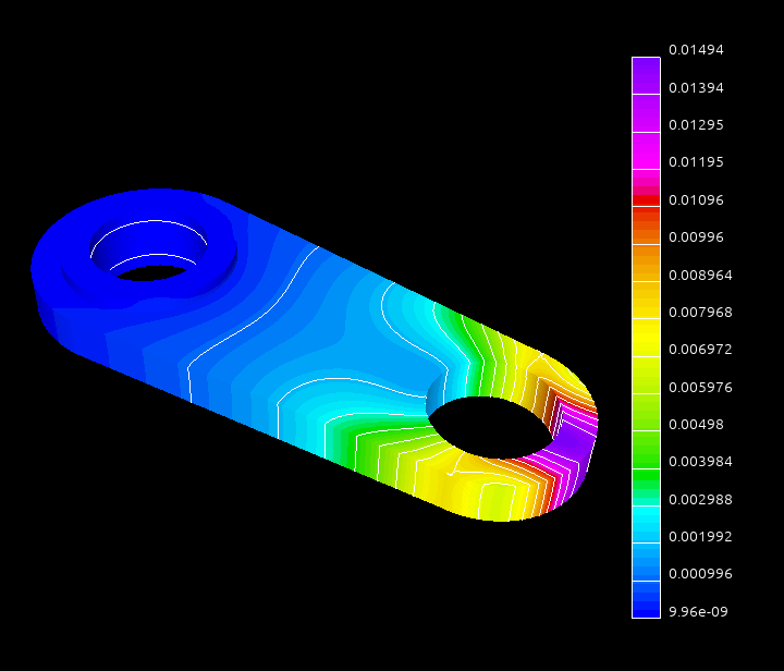
Fig. 8 The connecting rod geometry with the computed displacements
The dataset was kindly provided by David Herrero Pérez (@davidherreroperez) in the issue #135 on Github and is available for download at doi:10.5281/zenodo.4299865. The system matrix is symmetric, has block structure with small \(3\times3\) blocks, and has 81,657 rows and 3,171,111 nonzero values (about 39 nonzero entries per row on average). The matrix portrait is shown on the figure below:
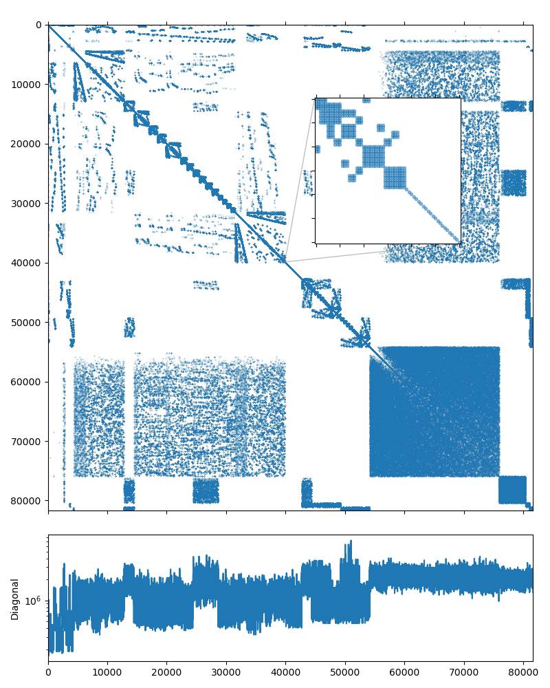
Fig. 9 The nonzero portrait of the connecting rod system.
It is possible to solve the system using the CG iterative solver preconditioned with the smoothed aggregation AMG, but the convergence is not that great:
$ solver -A A.mtx -f b.mtx solver.type=cg solver.maxiter=1000
Solver
======
Type:             CG
Unknowns:         81657
Memory footprint: 2.49 M

Preconditioner
==============
Number of levels:    3
Operator complexity: 1.14
Grid complexity:     1.07
Memory footprint:    70.09 M

level     unknowns       nonzeros      memory
---------------------------------------------
    0        81657        3171111     62.49 M (87.98%)
    1         5067         417837      7.16 M (11.59%)
    2          305          15291    450.07 K ( 0.42%)

Iterations: 698
Error:      8.96391e-09

[Profile:      11.717 s] (100.00%)
[  reading:     2.123 s] ( 18.12%)
[  setup:       0.122 s] (  1.04%)
[  solve:       9.472 s] ( 80.84%)
We can improve the solution time by taking the block structure of the system into account in the aggregation algorithm:
$ solver -A A.mtx -f b.mtx solver.type=cg solver.maxiter=1000 \
      precond.coarsening.aggr.block_size=3
Solver
======
Type:             CG
Unknowns:         81657
Memory footprint: 2.49 M

Preconditioner
==============
Number of levels:    3
Operator complexity: 1.29
Grid complexity:     1.10
Memory footprint:    92.40 M

level     unknowns       nonzeros      memory
---------------------------------------------
    0        81657        3171111     75.83 M (77.71%)
    1         7773         858051     15.70 M (21.03%)
    2          555          51327    890.16 K ( 1.26%)

Iterations: 197
Error:      8.76043e-09

[Profile:       5.525 s] (100.00%)
[  reading:     2.170 s] ( 39.28%)
[  setup:       0.173 s] (  3.14%)
[  solve:       3.180 s] ( 57.56%)
However, since this is an elasticity problem and we know the coordinates for
the discretization mesh, we can compute the rigid body modes and provide them
as the near null-space vectors for the smoothed aggregation AMG method. AMGCL
has a convenience function amgcl::coarsening::rigid_body_modes()
that takes the 2D or 3D coordinates and converts them into the rigid body
modes. The examples/solver utility allows to specify the file containing the
coordinates on the command line:
$ solver -A A.mtx -f b.mtx solver.type=cg \
      precond.coarsening.aggr.eps_strong=0 -C C.mtx
Solver
======
Type:             CG
Unknowns:         81657
Memory footprint: 2.49 M

Preconditioner
==============
Number of levels:    3
Operator complexity: 1.52
Grid complexity:     1.10
Memory footprint:    132.15 M

level     unknowns       nonzeros      memory
---------------------------------------------
    0        81657        3171111    102.70 M (65.77%)
    1         7704        1640736     29.33 M (34.03%)
    2          144           9576    122.07 K ( 0.20%)

Iterations: 63
Error:      8.4604e-09

[Profile:       3.764 s] (100.00%)
[  reading:     2.217 s] ( 58.89%)
[  setup:       0.350 s] (  9.30%)
[  solve:       1.196 s] ( 31.78%)
In the 3D case we get 6 near null-space vectors corresponding to the rigid body modes. Note that this makes the preconditioner more expensive memory-wise: the memory footprint of the preconditioner has increased to 132M from 70M in the simplest case and 92M in the case using the block structure of the matrix. But this pays up in terms of performance: the number of iterations dropped from 197 to 63 and the solution time decreased from 3.2 seconds to 1.2 seconds.
In principle, it is also possible to approximate the near null-space vectors by solving the homogeneous system \(Ax=0\), starting with a random initial solution \(x\). We may use the computed \(x\) as a near-null space vector, solve the homogeneous system again from a different random start, and do this until we have enough near null-space vectors. The examples/ns_search.cpp example shows how to do this. However, this process is quite expensive, because we need to solve the system multiple times, starting with a badly tuned solver at that. It is probably only worth the time in case one needs to solve the same system efficiently for multiple right-hand side vectors. Below is an example of searching for the 6 near null-space vectors:
$ ns_search -A A.mtx -f b.mtx solver.type=cg solver.maxiter=1000 \
      precond.coarsening.aggr.eps_strong=0 -n6 -o N6.mtx

-------------------------
-- Searching for vector 0
-------------------------
Solver
======
Type:             CG
Unknowns:         81657
Memory footprint: 2.49 M

Preconditioner
==============
Number of levels:    2
Operator complexity: 1.01
Grid complexity:     1.02
Memory footprint:    62.79 M

level     unknowns       nonzeros      memory
---------------------------------------------
    0        81657        3171111     60.56 M (98.58%)
    1         1284          45576      2.24 M ( 1.42%)

Iterations: 932
Error:      8.66233e-09

-------------------------
-- Searching for vector 1
-------------------------
Solver
======
Type:             CG
Unknowns:         81657
Memory footprint: 2.49 M

Preconditioner
==============
Number of levels:    2
Operator complexity: 1.01
Grid complexity:     1.02
Memory footprint:    62.79 M

level     unknowns       nonzeros      memory
---------------------------------------------
    0        81657        3171111     60.56 M (98.58%)
    1         1284          45576      2.24 M ( 1.42%)

Iterations: 750
Error:      9.83476e-09

-------------------------
-- Searching for vector 2
-------------------------
Solver
======
Type:             CG
Unknowns:         81657
Memory footprint: 2.49 M

Preconditioner
==============
Number of levels:    2
Operator complexity: 1.06
Grid complexity:     1.03
Memory footprint:    76.72 M

level     unknowns       nonzeros      memory
---------------------------------------------
    0        81657        3171111     68.98 M (94.56%)
    1         2568         182304      7.74 M ( 5.44%)

Iterations: 528
Error:      8.74633e-09

-------------------------
-- Searching for vector 3
-------------------------
Solver
======
Type:             CG
Unknowns:         81657
Memory footprint: 2.49 M

Preconditioner
==============
Number of levels:    3
Operator complexity: 1.13
Grid complexity:     1.05
Memory footprint:    84.87 M

level     unknowns       nonzeros      memory
---------------------------------------------
    0        81657        3171111     77.41 M (88.49%)
    1         3852         410184      7.42 M (11.45%)
    2           72           2394     31.36 K ( 0.07%)

Iterations: 391
Error:      9.04425e-09

-------------------------
-- Searching for vector 4
-------------------------
Solver
======
Type:             CG
Unknowns:         81657
Memory footprint: 2.49 M

Preconditioner
==============
Number of levels:    3
Operator complexity: 1.23
Grid complexity:     1.06
Memory footprint:    99.01 M

level     unknowns       nonzeros      memory
---------------------------------------------
    0        81657        3171111     85.84 M (81.22%)
    1         5136         729216     13.11 M (18.68%)
    2           96           4256     55.00 K ( 0.11%)

Iterations: 238
Error:      9.51092e-09

-------------------------
-- Searching for vector 5
-------------------------
Solver
======
Type:             CG
Unknowns:         81657
Memory footprint: 2.49 M

Preconditioner
==============
Number of levels:    3
Operator complexity: 1.36
Grid complexity:     1.08
Memory footprint:    114.78 M

level     unknowns       nonzeros      memory
---------------------------------------------
    0        81657        3171111     94.27 M (73.45%)
    1         6420        1139400     20.42 M (26.39%)
    2          120           6650     85.24 K ( 0.15%)

Iterations: 175
Error:      9.43207e-09

-------------------------
-- Solving the system
-------------------------
Solver
======
Type:             CG
Unknowns:         81657
Memory footprint: 2.49 M

Preconditioner
==============
Number of levels:    3
Operator complexity: 1.52
Grid complexity:     1.10
Memory footprint:    132.15 M

level     unknowns       nonzeros      memory
---------------------------------------------
    0        81657        3171111    102.70 M (65.77%)
    1         7704        1640736     29.33 M (34.03%)
    2          144           9576    122.07 K ( 0.20%)

Iterations: 100
Error:      8.14427e-09

[Profile:         48.503 s] (100.00%)
[  apply:          2.373 s] (  4.89%)
[    setup:        0.422 s] (  0.87%)
[    solve:        1.949 s] (  4.02%)
[  read:           2.113 s] (  4.36%)
[  search:        43.713 s] ( 90.12%)
[    vector 0:    12.437 s] ( 25.64%)
[      setup:      0.101 s] (  0.21%)
[      solve:     12.335 s] ( 25.43%)
[    vector 1:     9.661 s] ( 19.92%)
[      setup:      0.115 s] (  0.24%)
[      solve:      9.545 s] ( 19.68%)
[    vector 2:     7.584 s] ( 15.64%)
[      setup:      0.217 s] (  0.45%)
[      solve:      7.365 s] ( 15.18%)
[    vector 3:     6.137 s] ( 12.65%)
[      setup:      0.180 s] (  0.37%)
[      solve:      5.954 s] ( 12.28%)
[    vector 4:     4.353 s] (  8.97%)
[      setup:      0.246 s] (  0.51%)
[      solve:      4.100 s] (  8.45%)
[    vector 5:     3.541 s] (  7.30%)
[      setup:      0.337 s] (  0.69%)
[      solve:      3.200 s] (  6.60%)
[  write:          0.303 s] (  0.63%)
Note that the number of iterations required to find the next vector is
gradually decreasing, as the quality of the solver increases. The 6
orthogonalized vectors are saved to the output file N6.mtx and are also
used to solve the original system. We can also use the file with the
examples/solver:
$ solver -A A.mtx -f b.mtx solver.type=cg \
      precond.coarsening.aggr.eps_strong=0 -N N6.mtx
Solver
======
Type:             CG
Unknowns:         81657
Memory footprint: 2.49 M

Preconditioner
==============
Number of levels:    3
Operator complexity: 1.52
Grid complexity:     1.10
Memory footprint:    132.15 M

level     unknowns       nonzeros      memory
---------------------------------------------
    0        81657        3171111    102.70 M (65.77%)
    1         7704        1640736     29.33 M (34.03%)
    2          144           9576    122.07 K ( 0.20%)

Iterations: 100
Error:      8.14427e-09

[Profile:       4.736 s] (100.00%)
[  reading:     2.407 s] ( 50.83%)
[  setup:       0.354 s] (  7.47%)
[  solve:       1.974 s] ( 41.69%)
This is an improvement with respect to the version that only uses the blockwize structure of the matrix, but is about 50% less effective than the version using the grid coordinates in order to compute the rigid body modes.
The listing below shows the complete source code computing the near null-space
vectors from the mesh coordinates and using the vectors in order to improve the
quality of the preconditioner. We include the
<amgcl/coarsening/rigid_body_modes.hpp> header to bring the definition of
the amgcl::coarsening::rigid_body_modes() function in line 9, and
use the function to convert the 3D coordinates into the 6 near null-space
vectors (rigid body modes) in lines 65–66. In lines 37–38 we check that the
coordinate file has the correct dimensions (since each grid node has three
displacement components associated with the node, the coordinate file should
have three times less rows than the system matrix). The rest of the code should
be quite familiar.
1 2 3 4 5 6 7 8 9 10 11 12 13 14 15 16 17 18 19 20 21 22 23 24 25 26 27 28 29 30 31 32 33 34 35 36 37 38 39 40 41 42 43 44 45 46 47 48 49 50 51 52 53 54 55 56 57 58 59 60 61 62 63 64 65 66 67 68 69 70 71 72 73 74 75 76 77 78 79 80 81 82 83 84 85 86 87 88 89 90 91 92 93 | #include <vector>
#include <iostream>
#include <amgcl/backend/builtin.hpp>
#include <amgcl/adapter/crs_tuple.hpp>
#include <amgcl/make_solver.hpp>
#include <amgcl/amg.hpp>
#include <amgcl/coarsening/smoothed_aggregation.hpp>
#include <amgcl/coarsening/rigid_body_modes.hpp>
#include <amgcl/relaxation/spai0.hpp>
#include <amgcl/solver/cg.hpp>
#include <amgcl/io/mm.hpp>
#include <amgcl/profiler.hpp>
int main(int argc, char *argv[]) {
// The command line should contain the matrix, the RHS, and the coordinate files:
if (argc < 4) {
std::cerr << "Usage: " << argv[0] << " <A.mtx> <b.mtx> <coo.mtx>" << std::endl;
return 1;
}
// The profiler:
amgcl::profiler<> prof("Nullspace");
// Read the system matrix, the RHS, and the coordinates:
ptrdiff_t rows, cols, ndim, ncoo;
std::vector<ptrdiff_t> ptr, col;
std::vector<double> val, rhs, coo;
prof.tic("read");
std::tie(rows, rows) = amgcl::io::mm_reader(argv[1])(ptr, col, val);
std::tie(rows, cols) = amgcl::io::mm_reader(argv[2])(rhs);
std::tie(ncoo, ndim) = amgcl::io::mm_reader(argv[3])(coo);
prof.toc("read");
amgcl::precondition(ncoo * ndim == rows && (ndim == 2 || ndim == 3),
"The coordinate file has wrong dimensions");
std::cout << "Matrix " << argv[1] << ": " << rows << "x" << rows << std::endl;
std::cout << "RHS " << argv[2] << ": " << rows << "x" << cols << std::endl;
std::cout << "Coords " << argv[3] << ": " << ncoo << "x" << ndim << std::endl;
// Declare the solver type
typedef amgcl::backend::builtin<double> SBackend; // the solver backend
typedef amgcl::backend::builtin<float> PBackend; // the preconditioner backend
typedef amgcl::make_solver<
amgcl::amg<
PBackend,
amgcl::coarsening::smoothed_aggregation,
amgcl::relaxation::spai0
>,
amgcl::solver::cg<SBackend>
> Solver;
// Solver parameters:
Solver::params prm;
prm.precond.coarsening.aggr.eps_strong = 0;
// Convert the coordinates to the rigid body modes.
// The function returns the number of near null-space vectors
// (3 in 2D case, 6 in 3D case) and writes the vectors to the
// std::vector<double> specified as the last argument:
prm.precond.coarsening.nullspace.cols = amgcl::coarsening::rigid_body_modes(
ndim, coo, prm.precond.coarsening.nullspace.B);
// We use the tuple of CRS arrays to represent the system matrix.
auto A = std::tie(rows, ptr, col, val);
// Initialize the solver with the system matrix.
prof.tic("setup");
Solver solve(A, prm);
prof.toc("setup");
// Show the mini-report on the constructed solver:
std::cout << solve << std::endl;
// Solve the system with the zero initial approximation:
int iters;
double error;
std::vector<double> x(rows, 0.0);
prof.tic("solve");
std::tie(iters, error) = solve(A, rhs, x);
prof.toc("solve");
// Output the number of iterations, the relative error,
// and the profiling data:
std::cout << "Iters: " << iters << std::endl
<< "Error: " << error << std::endl
<< prof << std::endl;
}
|
The output of the compiled program is shown below:
$ ./nullspace A.mtx b.mtx C.mtx
Matrix A.mtx: 81657x81657
RHS b.mtx: 81657x1
Coords C.mtx: 27219x3
Solver
======
Type:             CG
Unknowns:         81657
Memory footprint: 2.49 M

Preconditioner
==============
Number of levels:    3
Operator complexity: 1.52
Grid complexity:     1.10
Memory footprint:    98.76 M

level     unknowns       nonzeros      memory
---------------------------------------------
    0        81657        3171111     76.73 M (65.77%)
    1         7704        1640736     21.97 M (34.03%)
    2          144           9576     61.60 K ( 0.20%)

Iters: 63
Error: 8.46024e-09

[Nullspace:     3.653 s] (100.00%)
[  read:        2.173 s] ( 59.48%)
[  setup:       0.326 s] (  8.94%)
[  solve:       1.150 s] ( 31.48%)
As was noted above, using the near null-space vectors makes the preconditioner less memory-efficient: since the 6 rigid-body modes are used as null-space vectors, every fine-grid aggregate is converted to 6 unknowns on the coarser level. The following figure shows the structure of the system matrix on the second level of the hierarchy, and it is obvious that the matrix has \(6\times6\) block structure:
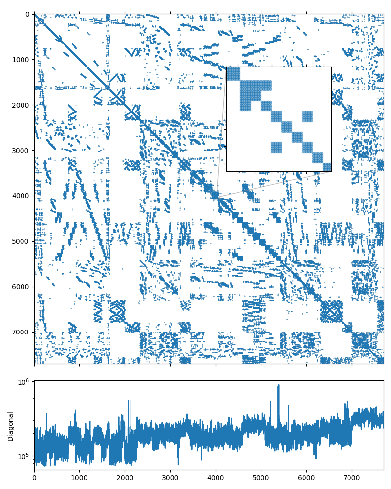
Fig. 10 The nonzero portrait of the system matrix on the second level of the AMG hierarchy.
It should be possible to represent both the initial matrix and the matrices on each level of the hiearachy using the \(3\times3\) block value type, as we did in the Structural problem example. Unfortunaltely, AMGCL is not yet able to utilize near null-space vectors with block-valued backends.
One possible solution to this problem, suggested by Piotr Hellstein (@dokotor) in GitHub issue #215, is to convert the matrices to the block-wise storage format after the hiearchy has been constructed. This has been implemented in form of the hybrid OpenMP and VexCL backends.
The listing below shows an example of using the hybrid OpenMP backend (tutorial/5.Nullspace/nullspace_hybrid.cpp). The only difference with the scalar code is the definition of the block value type and the use of the hybrid backend (lines 46–49).
1 2 3 4 5 6 7 8 9 10 11 12 13 14 15 16 17 18 19 20 21 22 23 24 25 26 27 28 29 30 31 32 33 34 35 36 37 38 39 40 41 42 43 44 45 46 47 48 49 50 51 52 53 54 55 56 57 58 59 60 61 62 63 64 65 66 67 68 69 70 71 72 73 74 75 76 77 78 79 80 81 82 83 84 85 86 87 88 89 90 91 92 93 94 95 96 | #include <vector>
#include <iostream>
#include <amgcl/backend/builtin_hybrid.hpp>
#include <amgcl/value_type/static_matrix.hpp>
#include <amgcl/adapter/crs_tuple.hpp>
#include <amgcl/make_solver.hpp>
#include <amgcl/amg.hpp>
#include <amgcl/coarsening/smoothed_aggregation.hpp>
#include <amgcl/coarsening/rigid_body_modes.hpp>
#include <amgcl/relaxation/spai0.hpp>
#include <amgcl/solver/cg.hpp>
#include <amgcl/io/mm.hpp>
#include <amgcl/profiler.hpp>
int main(int argc, char *argv[]) {
// The command line should contain the matrix, the RHS, and the coordinate files:
if (argc < 4) {
std::cerr << "Usage: " << argv[0] << " <A.mtx> <b.mtx> <coo.mtx>" << std::endl;
return 1;
}
// The profiler:
amgcl::profiler<> prof("Nullspace");
// Read the system matrix, the RHS, and the coordinates:
ptrdiff_t rows, cols, ndim, ncoo;
std::vector<ptrdiff_t> ptr, col;
std::vector<double> val, rhs, coo;
prof.tic("read");
std::tie(rows, rows) = amgcl::io::mm_reader(argv[1])(ptr, col, val);
std::tie(rows, cols) = amgcl::io::mm_reader(argv[2])(rhs);
std::tie(ncoo, ndim) = amgcl::io::mm_reader(argv[3])(coo);
prof.toc("read");
amgcl::precondition(ncoo * ndim == rows && (ndim == 2 || ndim == 3),
"The coordinate file has wrong dimensions");
std::cout << "Matrix " << argv[1] << ": " << rows << "x" << rows << std::endl;
std::cout << "RHS " << argv[2] << ": " << rows << "x" << cols << std::endl;
std::cout << "Coords " << argv[3] << ": " << ncoo << "x" << ndim << std::endl;
// Declare the solver type
typedef amgcl::static_matrix<double, 3, 3> DBlock;
typedef amgcl::static_matrix<float, 3, 3> FBlock;
typedef amgcl::backend::builtin_hybrid<DBlock> SBackend; // the solver backend
typedef amgcl::backend::builtin_hybrid<FBlock> PBackend; // the preconditioner backend
typedef amgcl::make_solver<
amgcl::amg<
PBackend,
amgcl::coarsening::smoothed_aggregation,
amgcl::relaxation::spai0
>,
amgcl::solver::cg<SBackend>
> Solver;
// Solver parameters:
Solver::params prm;
prm.precond.coarsening.aggr.eps_strong = 0;
// Convert the coordinates to the rigid body modes.
// The function returns the number of near null-space vectors
// (3 in 2D case, 6 in 3D case) and writes the vectors to the
// std::vector<double> specified as the last argument:
prm.precond.coarsening.nullspace.cols = amgcl::coarsening::rigid_body_modes(
ndim, coo, prm.precond.coarsening.nullspace.B);
// We use the tuple of CRS arrays to represent the system matrix.
auto A = std::tie(rows, ptr, col, val);
// Initialize the solver with the system matrix.
prof.tic("setup");
Solver solve(A, prm);
prof.toc("setup");
// Show the mini-report on the constructed solver:
std::cout << solve << std::endl;
// Solve the system with the zero initial approximation:
int iters;
double error;
std::vector<double> x(rows, 0.0);
prof.tic("solve");
std::tie(iters, error) = solve(A, rhs, x);
prof.toc("solve");
// Output the number of iterations, the relative error,
// and the profiling data:
std::cout << "Iters: " << iters << std::endl
<< "Error: " << error << std::endl
<< prof << std::endl;
}
|
This results in the following output. Note that the memory footprint of the preconditioner dropped from 98M to 41M (by 58%), and the solution time dropped from 1.150s to 0.707s (by 38%):
$ ./nullspace_hybrid A.mtx b.mtx C.mtx
Matrix A.mtx: 81657x81657
RHS b.mtx: 81657x1
Coords C.mtx: 27219x3
Solver
======
Type:             CG
Unknowns:         81657
Memory footprint: 2.49 M

Preconditioner
==============
Number of levels:    3
Operator complexity: 1.52
Grid complexity:     1.10
Memory footprint:    40.98 M

level     unknowns       nonzeros      memory
---------------------------------------------
    0        81657        3171111     31.90 M (65.77%)
    1         7704        1640736      9.01 M (34.03%)
    2          144           9576     61.60 K ( 0.20%)

Iters: 63
Error: 8.4562e-09

[Nullspace:     3.304 s] (100.00%)
[ self:         0.003 s] (  0.10%)
[  read:        2.245 s] ( 67.94%)
[  setup:       0.349 s] ( 10.57%)
[  solve:       0.707 s] ( 21.38%)
Another possible solution is to use a block-valued backend both for constructing
the hierarchy and for the solution phase. In order to allow for the coarsening
scheme to use the near null-space vectors, the
amgcl::coarsening::as_scalar coarsening wrapper may be used. The
wrapper converts the input matrix to scalar format, applies the base coarsening
strategy to the scalar matrix, and converts the computed transfer operators
back to block format. This approach results in faster setup times, since every
other operation besides coarsening is performed using block arithmetics.
The listing below shows an example of using the amgcl::coarsening::as_scalar
wrapper (tutorial/5.Nullspace/nullspace_block.cpp). The system matrix is
converted to block format in line 78 in the same way it was done in the
Structural problem tutorial. The RHS and the solution vectors are
reinterpreted to contain block values in lines 94-95. The SPAI0 relaxation here
resulted in the increased number of interations, so we used the ILU(0)
relaxaion.
1 2 3 4 5 6 7 8 9 10 11 12 13 14 15 16 17 18 19 20 21 22 23 24 25 26 27 28 29 30 31 32 33 34 35 36 37 38 39 40 41 42 43 44 45 46 47 48 49 50 51 52 53 54 55 56 57 58 59 60 61 62 63 64 65 66 67 68 69 70 71 72 73 74 75 76 77 78 79 80 81 82 83 84 85 86 87 88 89 90 91 92 93 94 95 96 97 98 99 100 101 102 103 104 105 106 | #include <vector>
#include <iostream>
#include <amgcl/backend/builtin.hpp>
#include <amgcl/value_type/static_matrix.hpp>
#include <amgcl/adapter/crs_tuple.hpp>
#include <amgcl/adapter/block_matrix.hpp>
#include <amgcl/make_solver.hpp>
#include <amgcl/amg.hpp>
#include <amgcl/coarsening/smoothed_aggregation.hpp>
#include <amgcl/coarsening/rigid_body_modes.hpp>
#include <amgcl/coarsening/as_scalar.hpp>
#include <amgcl/relaxation/ilu0.hpp>
#include <amgcl/solver/cg.hpp>
#include <amgcl/io/mm.hpp>
#include <amgcl/profiler.hpp>
int main(int argc, char *argv[]) {
// The command line should contain the matrix, the RHS, and the coordinate files:
if (argc < 4) {
std::cerr << "Usage: " << argv[0] << " <A.mtx> <b.mtx> <coo.mtx>" << std::endl;
return 1;
}
// The profiler:
amgcl::profiler<> prof("Nullspace");
// Read the system matrix, the RHS, and the coordinates:
ptrdiff_t rows, cols, ndim, ncoo;
std::vector<ptrdiff_t> ptr, col;
std::vector<double> val, rhs, coo;
prof.tic("read");
std::tie(rows, rows) = amgcl::io::mm_reader(argv[1])(ptr, col, val);
std::tie(rows, cols) = amgcl::io::mm_reader(argv[2])(rhs);
std::tie(ncoo, ndim) = amgcl::io::mm_reader(argv[3])(coo);
prof.toc("read");
amgcl::precondition(ncoo * ndim == rows && (ndim == 2 || ndim == 3),
"The coordinate file has wrong dimensions");
std::cout << "Matrix " << argv[1] << ": " << rows << "x" << rows << std::endl;
std::cout << "RHS " << argv[2] << ": " << rows << "x" << cols << std::endl;
std::cout << "Coords " << argv[3] << ": " << ncoo << "x" << ndim << std::endl;
// Declare the solver type
typedef amgcl::static_matrix<double, 3, 3> DBlock;
typedef amgcl::static_matrix<float, 3, 3> FBlock;
typedef amgcl::backend::builtin<DBlock> SBackend; // the solver backend
typedef amgcl::backend::builtin<FBlock> PBackend; // the preconditioner backend
typedef amgcl::make_solver<
amgcl::amg<
PBackend,
amgcl::coarsening::as_scalar<
amgcl::coarsening::smoothed_aggregation
>::type,
amgcl::relaxation::ilu0
>,
amgcl::solver::cg<SBackend>
> Solver;
// Solver parameters:
Solver::params prm;
prm.solver.maxiter = 500;
prm.precond.coarsening.aggr.eps_strong = 0;
// Convert the coordinates to the rigid body modes.
// The function returns the number of near null-space vectors
// (3 in 2D case, 6 in 3D case) and writes the vectors to the
// std::vector<double> specified as the last argument:
prm.precond.coarsening.nullspace.cols = amgcl::coarsening::rigid_body_modes(
ndim, coo, prm.precond.coarsening.nullspace.B);
// We use the tuple of CRS arrays to represent the system matrix.
auto A = std::tie(rows, ptr, col, val);
auto Ab = amgcl::adapter::block_matrix<DBlock>(A);
// Initialize the solver with the system matrix.
prof.tic("setup");
Solver solve(Ab, prm);
prof.toc("setup");
// Show the mini-report on the constructed solver:
std::cout << solve << std::endl;
// Solve the system with the zero initial approximation:
int iters;
double error;
std::vector<double> x(rows, 0.0);
// Reinterpret both the RHS and the solution vectors as block-valued:
auto F = amgcl::backend::reinterpret_as_rhs<DBlock>(rhs);
auto X = amgcl::backend::reinterpret_as_rhs<DBlock>(x);
prof.tic("solve");
std::tie(iters, error) = solve(Ab, F, X);
prof.toc("solve");
// Output the number of iterations, the relative error,
// and the profiling data:
std::cout << "Iters: " << iters << std::endl
<< "Error: " << error << std::endl
<< prof << std::endl;
}
|
This results are presented below. Note that even though the more advanced ILU(0) smoother was used, the setup time has been reduced, since ILU(0) was constructed using block arithmetics.:
$ ./nullspace_block A.mtx b.mtx C.mtx
Matrix A.mtx: 81657x81657
RHS b.mtx: 81657x1
Coords C.mtx: 27219x3
Solver
======
Type:             CG
Unknowns:         27219
Memory footprint: 2.49 M

Preconditioner
==============
Number of levels:    3
Operator complexity: 1.52
Grid complexity:     1.10
Memory footprint:    63.24 M

level     unknowns       nonzeros      memory
---------------------------------------------
    0        27219         352371     46.45 M (65.77%)
    1         2568         182304     16.73 M (34.03%)
    2           48           1064     60.85 K ( 0.20%)

Iters: 32
Error: 7.96226e-09

[Nullspace:     2.885 s] (100.00%)
[  read:        2.160 s] ( 74.87%)
[  setup:       0.249 s] (  8.64%)
[  solve:       0.473 s] ( 16.39%)